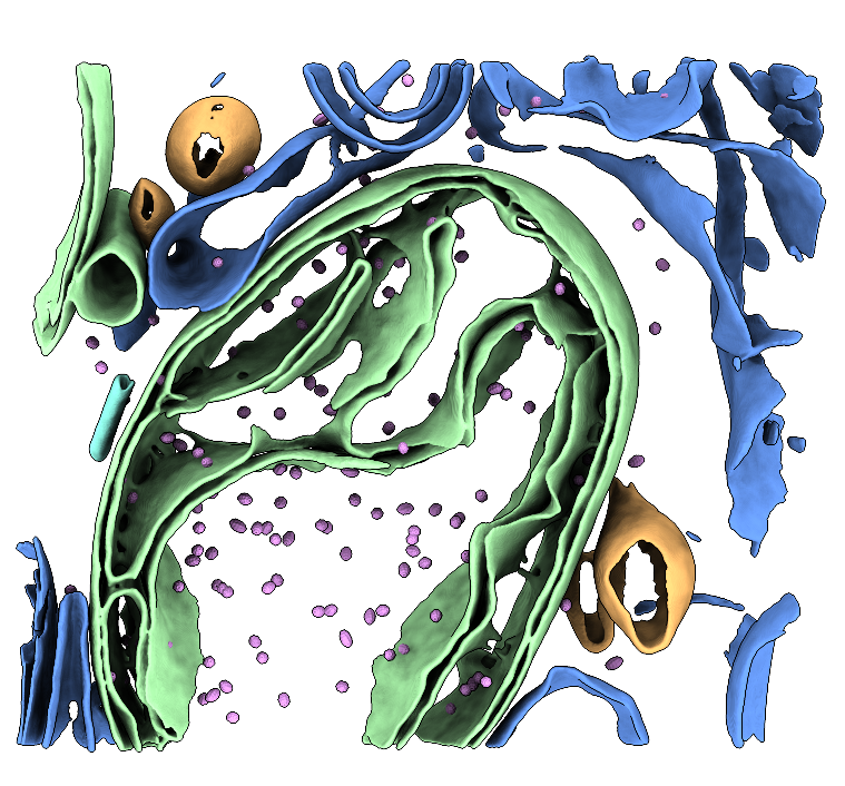
Two raw tilt-series (in MRC format) of FIB-milled G-TPP-treated HeLa cells that have been milled. The dataset contains mitochondria and cytoplasmic ribosomes as well as mHSP60-mHSP10 chaperonin "football" complexes. MRC files and MDOC files are provided. See the Processing Bundle below for all the scripts necessary to reconstruct the data to low-resolution following our tutorial. This tutorial involves template matching, subtomogram averaging, membrane segmentation, and particle place-back. See the processing instruction document for full details. Storage required: 4.4 G (dataset size) and 50G (storage for processing files when the tutorial has been completed).
Data DOI: 10.15785/SBGRID/1273 | Publication DOI: 10.1101/2025.10.06.680693 | Published: 10 Jul 2026
Ruben Fernandez-Busnadiego, University of Göttingen
Cells have evolved organelle-specific strategies to preserve protein homeostasis. In mitochondria, proteostatic stress suppresses protein synthesis and promotes protein folding, but the structural basis of these responses is not well understood. Using cryo-electron tomography, the authors examined how mitochondrial proteostatic stress alters cellular ultrastructure in human cells. They observed protein aggregates within the mitochondrial matrix together with extensive remodeling of cristae architecture. At the same time, the mitochondrial chaperonin Hsp60 (mHsp60), a central folding machine, exhibited pronounced conformational changes that favored association with its co-chaperone mHsp10. The authors directly visualized mHsp60 interactions with native substrate proteins in situ and determined cryo-EM structures of mHsp60 in vitro, allowing assignment of nucleotide states to the cellular complexes. These results supported a model for the mHsp60 functional cycle and highlight its essential role in maintaining mitochondrial proteostasis.
Note: This tutorial dataset is small and has a limited number of Hsp60 molecules available. After subtomogram averaging (STA), your resulting reconstruction will be low-resolution. However, you will still reconstruct tomograms, segment membranes and microtubules, perform template matching and learn how to convert file formats, verify particle coordinates, and carry out low-resolution STA. In principle, these skills would enable you to reproduce the authors’ results on the full-sized dataset.
Author information: Ehses K, López-Alonso JP, Antico P, Azem A, Muqit MM, Ubarretxena-Belandia I, Fernández-Busnadiego R.
DOI: 10.1101/2025.10.06.680693
EMPIAR deposition: EMPIAR-13145
ChallengeBank deposition: 10.15785/SBGRID/1273
Why this dataset is challenging:
/warp_tiltseries/ folder.Time to completion: ~1–2 days
Computing required: This guide was made with the intention that an investigator will have access to 2-4 GPUs with at least 16GB of VRAM each. More GPUs is certainly better, and less will mean processing will take longer than the time estimates provided in this guide. Ultimately, we leave the computing power dedicated to this tutorial to the discretion of the investigator.
Storage required: 4.4 G (dataset size) and 50G (storage for processing files).
Software suggested: Multiple software packages need to be used to complete the entire reconstruction. Investigators are welcome to complete as little or as much of the reconstruction pipeline as desired, and pre-calculated results are available if you would prefer to skip certain steps.
For this dataset, we recommend Relion (5.0.0_cu12.2), Imod/3Dmod (4.11.25), MemBrain (version 0.0.9), Pytom-match-pick (1.1), UCSF ChimeraX (version 1.10_rhel9) and the ArtiaX plug-in for UCSF ChimeraX (1.3).
This dataset contains 2 tilt-series of focus-ion beam milled virally-infected cells. For reconstructing a fully annotated tomogram series, we recommend a full pipeline inclusive of membrane segmentation, particle localization and template matching, subtomogram averaging and latent space classing. You have the optional step of tomogram deconvolution as an alternative to denoising to sharpen features of the tomograms.
We will be following the 8 basic steps of tomographic reconstruction:
If you have not already downloaded the data, open a command terminal window and type the following command:
rsync -av rsync://challengebank.sbgrid.org/10.15785/SBGRID/1273Check the integrity of the download by assessing if all the components are correctly downloaded to your computer. This pack should contain motion-corrected .mrc tilt images, .mdocs, and a copy of these instructions.
New tomographers are often confused about the difference between a frame series, a movie, a micrograph and a tilt series. If you know these terms, skip to the next page. If you’re unsure, keep reading.
When a dataset is collected on the microscope, a short movie is taken by exposing the sample to a certain dose of electrons over a certain period of time. The dose is fractionated into frames over the time taken to collect the movie. The movie is therefore composed of a series of frames, called a frame series. The sample stage is then tilted in the microscope in preparation for collecting the next movie (or frame series). At the end of data collection, you will have a collection of movies, each taken at a different discrete angle. The collection of frame series acquired across the tilt range constitutes the raw tilt-series data. After motion correction and summing, each frame series yields one tilt image (micrograph). The ordered set of tilt images acquired at discrete angles is the tilt series.
Create a workspace. Before we begin, we need to set up a clean workspace for us to be able to work from.
mkdir relion_sbchallenge to make a new directory called “relion_sbchallenge”cd relion_sbchallenge to move into the new directoryln -s /path/to/tutorial/data ./ to create a link to your dataConcept: In WarpTools, correct for a) motion blur that occurred during data collection, b) the CTF gradient that causes high frequency information loss in an uneven way across the images as they are progressively tilted relative to the electron beam, and c) remove bad frames from our tilt-series. We will then align the tilt-series with AreTomo3 and erase the gold fiducials with Fidder. Reconstruction will take place using WarpTools.
This dataset will be reconstructed in WarpTools, the Linux-version of Warp.
IMPORTANT: File housekeeping before tilt-series import later
Because the data are already motion-corrected, we skipped the motion correction job and went directly to the CTF estimation job. We now have to do some file housekeeping that would have occurred during the motion correction job. During the motion correction job, WarpTools stores summed average tilts in .mrc format in a newly created /average/ folder, found at warp_frameseries/average/. We already have these images, but because we didn’t run the motion correction job, the directory was never made. WarpTools needs these summed averages at the tilt-series import step. We must make the directory ourselves and then symbolically link the summed averages to that location.
How to symbolically link your motion corrected tilt series:
/warp_tiltseries/ directory.
cd warp_tiltseriesln -s /path/to/data//data/) to the name that WarpTools expects, which is /average/.
mv data average/average/ directory now. You should see all the frames printed to the terminal.
ls averageWarpTools create_settings \
--output warp_frameseries.settings \
--folder_processing /PATH/TO/YOUR/WORKING/DIRECTORY/warp_frameseries \
--folder_data /PATH/TO/YOUR/DATA/ \
--extension "*.mrc" \
--angpix 2.31 \
--bin 0 \
--exposure 3.69 \
--tomo_dimensions 4400x4400x2200 > 1_warp_create_fs_settings.out 2> 1_warp_create_fs_settings.errThis script will create a file called warp_frameseries.settings that will be stored in your project directory. This file is a type of XML metadata file that supplies WarpTools with the settings you provided. If you are curious, we encourage you to open the file in a text editor and check out what’s inside it.
In your script:
warp_frameseries.settings./$path/$to/$your/$data/warp_frameseries/$path/$to/$your/$data/*.mrc.Time to run (run directly in the commandline): Nearly instant.
Note: Because the data are already motion-corrected, we have skipped motion-correction.
WarpTools fs_ctf \
--settings warp_frameseries.settings \
--voltage 300 \
--cs 2.7 \
--amplitude 0.1 \
--defocus_min 3.0 \
--defocus_max 8.0 \
--range_min 30.0 \
--range_max 5.0 \
--use_sum \
--grid 2x2x1 > 2_warp_fs_ctf.out 2> 2_warp_fs_ctf.err
This script will run the CTF estimation job in WarpTools. You will notice that the /warp_frameseries/ folder has appeared. If you look at the contents of that folder, you’ll see an .xml file for every motion-corrected tilt in our dataset.
In your script:
Time to run (on 4 GPUs): ~5 minutes
WarpTools filter_quality \
--settings warp_frameseries.settings \
--histograms > 3_warp_histograms.out 2> 3_warp_histograms.err
This script will print histograms to the terminal screen that will allow you to determine if the motion correction and CTF estimation completed as expected. It can be difficult to tell if the histograms are depicting something sensible, so a good rule of thumb is to look for a normal bell-shape distribution across the defocus. We know that we should expect a normal distribution because the sample was progressively tilted in the microscope, so defocus should progressively increase. In our experience, if something has gone wrong at this stage, WarpTools tends to dump all frames into the last value of the histograms.
In your script:
Time to run (run in the terminal): Nearly instant.
WarpTools ts_import \
--mdocs /path/to/edited/mdoc/ \
--pattern "*mdoc" \
--frameseries warp_frameseries \
--tilt_exposure 3.69 \
--dont_invert \
--override_axis 85 \
--output tomostar \
--min_intensity 0.8 > 4_warp_ts_import.out 2> 4_warp_ts_import.err
WarpTools needs to import the single frame tilts using an mdoc file so that WarpTools can know what angle each summed tilt was imaged at. Mdoc files record the angle of each frame series, and since the tilt series have the same file name, WarpTools is able to determine the associated tilt angle.
In your script:
.tomostar files. This folder doesn’t exist yet, but WarpTools will make it for you after this job has been completed. (Here: tomostar.).tomostar file for each tilt series. You can run this job with some value like 0.3, and check the tomostar files afterwards, or you can make a conservative guess and try a few values until you achieve good results. In our case, we don’t have any dark frames, so it doesn’t matter.Time to run (run in the terminal): Nearly instant.
WarpTools create_settings \
--output warp_tiltseries.settings \
--folder_processing warp_tiltseries \
--folder_data tomostar \
--extension "*.tomostar" \
--angpix 2.31 \
--bin 0 \
--exposure 3.69 \
--tomo_dimensions 4400x4400x2200 > 5_warp_ts_settings.out 2> 5_warp_ts_settings.err
This script will create a settings file that defines the relevant parameters related to the tilt series. The settings are all the same. If you wanted to bin your pixel size, but you didn’t bin it from the start, now would be your chance to bin the pixel size to speed up processing.
In your script:
warp_tiltseries.settings.*.tomostar.Time to run (run in the terminal): Less than a minute.
6_warptools_stack.sh
WarpTools ts_stack \
--settings warp_tiltseries.settings \
--angpix 10 \
--output_processing stack > 6_warp_stack.out 2> 6_warp_stack.err
This script will stack our motion-corrected MRC files into the order that they should be viewed in (rather than in the order that they were collected in) by using the tilt information from the tomostar file. This stack will be placed in a folder called /stack/ within our working directory.
Next, we will create a text file that lists the tilts we wish to exclude from downstream processing. To do this, we need to view our stacked images, decide which tilts to be excluded and place their file names in a text file. Stacked MRC files do not retain the image names for the slices they are composed of, so all the tilts have been renumbered and no longer correspond to their original index numbers as recorded in the MDOC file. Instead, they now are simply renumbered based on the order from highest positive tilt angle to highest negative tilt angle.
To identify the name of the tilt which needs to be removed, we can use the tomostar files to help us. If you are confused, please watch the YouTube tutorial associated with this dataset. To do this, we need to do a few things:
imod stack/tiltstack/$TOMO/$TOMO.stexclude_list.txt. We will need this text file soon.
geany exclude_list.txt(or a text editor of your choice)
/tomostar/. It is important that you use a text editor that has line numbers.HeLa_end_4hGTPP_139_009.st file is corrupted. This tilt must be excluded. When viewed in IMOD, the tilt appears on slice 27.HeLa_end_4hGTPP_139_009.tomostar, the line corresponding to the unwanted tilt is equal to the slice number from IMOD + 10. Since we don’t want tilt 27, you can find the image name on line 37 of the tomostar file. Copy the image name and paste it into exclude_list.txt.exclude_list.txt, provide the path to your data folder in front (on our machine, that folder is called /data/). In the end, you should have a text file that has one MRC file name per line, as per our example below.exclude_list.txt
data/HeLa_end_4hGTPP_139_170_42.0_Oct19.mrc
data/HeLa_end_4hGTPP_139_305_63.0_Oct19.mrc
data/HeLa_end_4hGTPP_139_314_66.0_Oct19.mrc
data/HeLa_end_4hGTPP_139_298_63.0_Oct19.mrcTo deselect our unwanted frames, we must first select all the frames in our dataset. After selecting all the frames, we then point WarpTools to our exclude_list.txt file, which will set an unselection flag in the corresponding xml file of any tilts we do not want.
Note: Please note that change_selection tool in WarpTools dev39 currently outputs unusual log files which do not accurately reflect the number of frames selected/deselected. For this job, we recommend you ignore the log files.
7_warptools_select_frames.sh
WarpTools change_selection \
--settings warp_frameseries.settings \
--select > 7_warp_select.out 2> 7_warp_select.err

WarpTools change_selection \
--settings warp_frameseries.settings \
--deselect --input_data exclude_list.txt > 7_warp_deselect.out 2> 7_warp_deselect.err8_update_mdoc.sh
python3 remove_excluded_tilts_from_mdoc.py data/*.mdoc \
--exclude exclude_list.txt \
--out clean_mdocs
This step will use a Python script (link below) to remove unwanted frames from our MDOC files. The edited MDOC files will be stored in a new subdirectory called /clean_mdocs/.
GitHub link: https://github.com/aeruera/Cryo-ET_Mdoc_Management_Scripts/blob/main/remove_excluded_tilts_from_mdoc.py
9_warptools_ts_import_update.sh
WarpTools ts_import \
--mdocs clean_mdocs \
--pattern "*.mdoc" \
--frameseries warp_frameseries \
--tilt_exposure 3.69 \
--override_axis 85 \
--output tomostar \
--min_intensity 0.8 > 9_warp_ts_import_update.out 2> 9_warp_ts_import_update.err
We should now have all the xml files referencing our unwanted frames with a flag at the top indicating UnselectManual = True, and new tomostar files which do not reference the unwanted frames.
10_warptools_align_aretomo3.sh
WarpTools ts_aretomo3 \
--settings warp_tiltseries.settings \
--angpix 10 \
--patches 6,5
WarpTools has a wrapper for the fiducial-free alignment tool AreTomo3. (Although this dataset does contain gold fiducial markers, when we benchmarked alignment with Etomo and AreTomo3, we found that AreTomo3 performed better on this dataset despite the presence of fiducial markers.)
In your script:
Time to run (on 4 GPUs): ~5 minutes.
Next, we will erase the gold fiducial markers from our images. Due to extremely high contrast, gold fiducials create strange streak artifacts in tomograms and can also confuse particle picking tools.
Note: Because we have SBGrid installed, we simply run Fidder as reported below because Fidder is pre-configured with the pre-trained model provided by the software developers. If you installed Fidder yourself, you may need to point the tool to the model on your machine.
11_fidder_erase_gold.sh
mkdir -p warp_frameseries/fidder_masks
mkdir -p warp_frameseries/fidder_edit
for f in warp_frameseries/average/*.mrc; do
base=$(basename "$f" .mrc)
fidder predict \
--input-image "$f" \
--probability-threshold 0.5 \
--pixel-spacing 2.31245 \
--output-mask "warp_frameseries/fidder_masks/${base}_mask.mrc"
fidder erase \
--input-image "$f" \
--input-mask "warp_frameseries/fidder_masks/${base}_mask.mrc" \
--output-image "warp_frameseries/fidder_edit/${base}.mrc"
doneThis tool will identify gold fiducials in our dataset by looking for high contrast peaks in the images and creating a mask around them. The mask is then used to “erase” the gold fiducials by back-filling the fiducial region with grey values similar to grey values in the neighbouring voxels of the image. Gold-erased images are stored in /warp_frameseries/fidder_edit/.
WarpTools expects the images for tomogram reconstruction to come from the /average/ folder in the /warp_frameseries/ directory. Currently, that folder contains our old images that still contain gold fiducial markers. We simply need to rename the current /average/ folder to something else, and rename the /fidder_edit/ folder to /average/.
11.1 Move into the /warp_frameseries/ folder.
cd warp_frameseries11.2 Rename the /average/ folder to something else, such as /original_average/.
mv average original_average11.3 Rename the /fidder_edit/ folder to /average/.
mv fidder_edit average11.4 Return to the working directory one level up on the system.
cd ..WarpTools ts_defocus_hand \
--settings warp_tiltseries.settings \
--check > 12_warp_check_defocus.out 2> 12_warp_check_defocus.errThis script will compute whether the defocus handedness of the data correlates with the expected CTF model. The result of this quick test will tell us if we need to change any settings related to the defocus handedness.
Read the results of this job in the log.
Time to run (run in the terminal): Nearly instant.
WarpTools ts_defocus_hand \
--settings warp_tiltseries.settings \
--set_noflip > 13_warp_set_defocus.out 2> 13_warp_set_defocus.err
This script will change our settings so that the defocus handedness is flipped.
Time to run (run in the terminal): Nearly instant.
WarpTools ts_ctf \
--settings warp_tiltseries.settings \
--defocus_min 3.0 --defocus_max 8.0 \
--range_low 30.0 --range_high 5.0 \
--voltage 300 --cs 2.7 --amplitude 0.1
This script performs 3D CTF correction using the 2D CTF estimation job for the frame series as an initial estimate.
In your script:
All parameters are the same as in our previous CTF estimation job.
Time to run (run in the terminal): Nearly instant.
WarpTools ts_reconstruct \
--settings warp_tiltseries.settings \
--angpix 10.00 \
--dont_invert \
--deconv \
--deconv_strength 0.7 \
--deconv_falloff 0.7 \
--perdevice 1
This script will reconstruct the tomogram by direct Fourier-inversion using the alignment information in the .xf file from our AreTomo3 job, the settings stored in the tilt series settings file (tomogram dimensions, etc), and the images in our recently edited /average/ folder.
In your script:
Time to run (run in the terminal): Nearly instant.
Now that you have a tomogram, you need to check that it looks as expected. To do this, open the tomogram in IMOD by typing imod tomoname.mrc from within the directory where the tomogram is stored. An info box should appear and a Zap viewing window.
You can scroll through the Z-stack of the image by sliding the Z slicer to the right and left. You’ll see mitochondrial membranes, cristae, and other cellular features.
Please rename your tomograms to remove the _10.00Apx pixel size suffix. You can do this now, or just before template matching, as long as you don’t forget. If you leave the pixel size suffix in the tomogram name, _10.00Apx will make its way into the STAR file when pytom-match-pick extracts particles. You’ll have to edit the STAR file later to remove it.
Concept: Use automated tools to create binary masks that represent the surfaces of membranes or other cellular components within the tomogram. This dataset contains both mitochondrial membrane surfaces, golgi and microtubules, all of which can be segmented rather well using automated tools. In our hands, MemBRAIN-seg performs best for segmenting surfaces and TARDIS performs better for segmenting microtubules.
For this tutorial, we will use an automated segmentation tool called MemBRAIN-seg to segment the membrane surface of mitochondria and other vesicles. This segmentation will help us with visualization later.
1_membrain.sh
membrain segment \
--tomogram-path /path/to/tomoname.mrc \
--ckpt-path /path/to/MemBrain_seg_v10_beta.ckpt \
--out-folder .
IMPORTANT: --tomogram-path needs a full path and must include the name of the tomogram. It cannot parse relative paths.
In your script:
This script will direct MemBRAIN-seg to the location on your system where the MemBRAIN pre-trained model is stored (the .ckpt file) and the tomogram you wish to segment. You must supply the full absolute path to the tomogram and remember to include the tomogram name.
Time to run (run in the terminal): 15 minutes
1.1 To view your segmentation, first load your file into UCSF ChimeraX:
chimerax membrain-seg/HeLa_end_4hGTPP_139_002_MemBrain_seg_v10_beta.ckpt_segmented.mrc1.2 In the Volume Viewer, set the render style to SURFACE, set the LEVEL to 0.1 and the STEP to 1.
1.3 In the command line within the ChimeraX GUI, type “surface smooth #1 factor 0.2 iterations 10”.
1.4 In the Model Viewer, unclick the original volume so that only the smoothed surface volume is visible.
1.5 Adjust the lighting to make the segmentation more pleasing to the eye and increase the sense of a depth of view. The SOFT lighting option is very popular in the cryoEM community in general. Silhouette will also help define the edges. Both options are available in the Graphics tab at the top of the GUI.
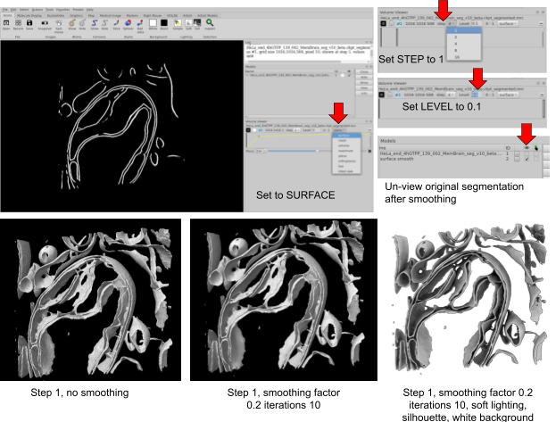
You will see that since this volume is a semantic segmentation, you have no control over individual colour or render settings for different features in the segmentation. You can apply only one colour to the whole file and you cannot blink off or un-show any regions at will.
We will split this file into a instance segmentation next.
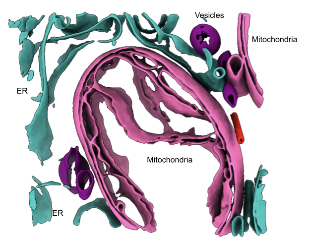
The memBRAIN-seg output is a semantic segmentation, meaning that all segmented features are treated as a single binary structure. For downstream analysis, we want to generate instance segmentations, where each feature is treated as a separate object and is only considered connected to another feature if they share connected voxels. To convert the semantic segmentation into an instance segmentation, we will use a Python script.
python3 split_semantic_mrc_into_instances.py \
--output_dir instances \
--connectivity 26 \
--min_voxels 600 \
--cropped --write_chimerax_script \
$segmentation.mrc
GitHub link:
You will have a .cxc file stored in /instances/ which can be directly opened in UCSF ChimeraX using chimerax open_instances_with_origins.cxc. Open this in ChimeraX the same way you did for the original semantic segmentation. You can now hide or show features at will and colour features however you please.
Concept: Learn how to create templates and masks for running Pytom-match-pick. Localize particles using the template and mask you create and then visualize particle locations in ArtiaX to make a quality assessment. Edit STAR files to make them compatible with WarpTools.
You may choose to symbolically link your /reconstruction/ folder inside your pytom-match-pick folder. Otherwise, edit the paths in the scripts below where the tomogram path is called for.
(We also provide the template and mask for your convenience so feel free to skip this step if you are not interested and proceed to 3. Template matching.) We need an initial 3D volume to begin. Ideally, this would be generated from your own data by manually picking enough particles to produce a low-resolution reconstruction, which can then be used as a template for template matching. In practice, however, many investigators use an existing structure as the template, since it saves time and manual effort. Using a pre-existing structure can substantially speed up processing since you can skip the step of producing it yourself. In this case, we will use a structure from EMD-54898: https://www.ebi.ac.uk/emdb/EMD-54898.
wget https://ftp.ebi.ac.uk/pub/databases/emdb/structures/EMD-54898/map/emd_54898.map.gzThis command downloads the volume map from EMD-54898 and saves a zipped file to the current directory.
ls and confirm that you see emd_54898.map.gz in the working directory.gunzip emd_54898.map.gz..map file to a .mrc file (pytom-match-pick cannot recognize .map file extensions):
mv emd_54898.map emd_54898.mrcls.1_create_template.sh
pytom_create_template.py \
-i emd_54898.mrc \
-o hsp60_football_template_54898.mrc \
--input-voxel-size-angstrom 0.8238 --output-voxel-size-angstrom 10 \
--center --log info --invert
In your script:
This command is very light and can be run directly in the command line.
Time to run (0 GPUs): a few seconds.
2.1 Check the box size of the new template. In Step 2, we will create an asymmetrical mask to encompass the template. Before we can do that, we need to check what box size pytom-match-pick has selected for the template. We need this value for Step 3.
header hsp60_football_template_54898.mrc. You should see the following:

Our box size is therefore 49 pixels for all dimensions.
2_Create_mask.sh
pytom_create_mask.py \
-b 49 \
-o hsp60_mask.mrc \
--voxel-size 10 -r 10 --radius-minor1 10 --radius-minor2 15 \
--s 0.5
In your script:
This command is very light and can be run directly in the command line.
Time to run (0 GPUs): a few seconds.
Pytom-match-pick needs to be run in a “for” loop in order to template match on multiple tomograms. It won’t run if you try to use Linux wildcards. We provide the for loop below, along with a suggested Slurm template for those using a resource cluster. You will need to adjust the Sbatch parameters to be suitable on your system. You need to edit the directory paths highlighted in yellow to match the directory on your machine.
Alternatively, since we have only two tomograms, you can simply run the script twice (once for each tomogram) so that pytom-match-pick will template match on them simultaneously. Of course, this only works for micro-datasets like this one, but this is just a tutorial, after all. We leave the run decisions up to you.
3_match_template.sh
#!/bin/bash

#SBATCH --ntasks=1
#SBATCH --nodes=1
#SBATCH --cpus-per-task=12
#SBATCH --gres=gpu:4
#SBATCH --partition=em-gpu
#SBATCH --error=logs/pytom_match_template.err
#SBATCH --output=logs/pytom_match_template.out
#SBATCH --job-name=pytom-match-pick

PYTOM_DIR="."
TEMPLATE="hsp60_football_template_54898.mrc"
MASK="hsp60_mask.mrc"

TOMO_DIR=" ../1_warptools/warp_tiltseries/reconstruction "
TILTSTACK_DIR=" ../1_warptools/warp_tiltseries/tiltstack "

OUT_DIR="${PYTOM_DIR}"

mkdir -p logs
mkdir -p "$OUT_DIR"

for tomo in "$TOMO_DIR"/*.mrc; do
# Handle case where no .mrc files are found
if [ ! -e "$tomo" ]; then
echo "No .mrc files found in $TOMO_DIR"
break
fi
tomo_file=$(basename "$tomo")
base="${tomo_file%.mrc}"

# rec_PR8-TS22 -> PR8-TS22
ts="${base#rec_}"

# Example of an expected WarpTools raw tilt file:
# ../1_warptools/warp_tiltseries/tiltstack/PR8-TS22/PR8-TS22.rawtlt
angles="${TILTSTACK_DIR}/${ts}/${ts}.rawtlt"

dest="${OUT_DIR}/${base}"

echo "----------------------------------------"
echo "Processing tomogram: $tomo"
echo "Using angles: $angles"
echo "Output directory: $dest"
echo "----------------------------------------"

if [ ! -f "$tomo" ]; then
echo "Missing tomogram: $tomo"
continue
fi
if [ ! -f "$angles" ]; then
echo "Missing angle file: $angles"
echo "Skipping $tomo_file"
continue
fi
mkdir -p "$dest"

pytom_match_template.py \
-t "$TEMPLATE" \
-v "$tomo" \
-d "$dest" \
-m "$MASK" \
--particle-diameter 150 \
--angular-search 10 \
--non-spherical-mask \
-a "$angles" \
--random-phase-correction \
-s 2 2 1 \
--voxel-size-angstrom 10 \
--high-pass 400 \
--tomogram-ctf-model phase-flip \
--per-tilt-weighting \
-g 0 1 2 3 \
--log info
done
In your script:
The results will be stored inside /pytom_outputs/TOMONAME/ with a separate folder for each tomogram.
Submit with sbatch 3_template_match.sh.
Time to run (4 GPUs): ~2 hours if run in a for loop, ~1 hour if run as two separate jobs in parallel
We want to extract particles that are not too close to the edge of the tomogram. Particles that are too close to the edge may have a truncated part of the particle box. The part of a truncated particle box where there is no biological signal is filled with stripe noise, which is very very bad for 3D reconstruction. To prevent this, we can create a border mask which masks out the edge of our tomogram. Only particles inside the border will be extracted.
We have a Python script for this task. To run it, simply run:
./make_boundary_mask.py /$path/$to/$tomogram.mrc --margin-angstrom 500This will save a mask with the same dimensions as your tomogram into the working directory with a border that is 500 angstroms inside the tomogram.
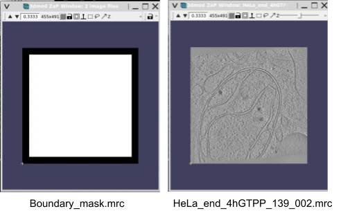
Now we can extract particle positions into a Relion 5 compatible STAR file for visualization in UCSF ChimeraX.
4_extract_particles.sh
pytom_extract_candidates.py -j HeLa_end_4hGTPP_139_002_job.json \
--particle-diameter 170 -n 150 --relion5-compat --c 0.38 --tomogram-mask boundary_mask.mrc

pytom_extract_candidates.py -j HeLa_end_4hGTPP_139_009_job.json \
--particle-diameter 170 -n 150 --relion5-compat --c 0.38 --tomogram-mask boundary_mask.mrc
Note: You may need to adjust the --c to lower it for less restrictive extraction.
This command is very light and can be run directly in the command line with ./4_extract_particles.sh.
Time to run (0 GPUs): <1 minute
These STAR files can then be loaded into ArtiaX for visualization.
5.1 Launch UCSF ChimeraX. If you have the app on your desktop, launch it by clicking the icon, or otherwise, in the terminal simply type chimerax.
5.2 Click on the ARTIAX tab at the top

5.3 Click on the LAUNCH button and select the tomogram from your /1_warptools/warp_tiltseries/reconstruction/ folder
Note: If the tomogram loads with an odd render appearance and is very pixelated, you might need to invert the contrast using the Invert Contrast button on the right hand tomogram menu. This sometimes happens occasionally and inverting the contrast seems to fix the bad pixelation. You can either continue viewing the tomogram with an inverted contrast or otherwise you can invert it a second time to restore the original contrast settings of dark particles on a light background.
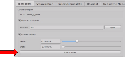
5.4 Under Particles List, select Open List.
5.4.1 Browse for the HeLa_end_4hGTPP_139_002_particles.star file
5.4.2 An Additional Information box will appear. Use the Drop Down bar to select the tomogram we are currently viewing.
5.4.3 In the Prefix box, put the tomogram prefix WITHOUT the tomogram unique identifier number. For example, if the tomogram is ‘HeLa_end_4hGTPP_139_002’, then the prefix is ‘HeLa_end_4hGTPP_139_00’ (without the final 2).
Navigate around the tomogram and make sure that the particle axes markers seem to fit over a density that reflects our expectations. What you don’t want to see is a marker over membranes, ice contaminants, or over specimens that are obviously not what we template matched for. Close ChimeraX once you are satisfied.
When you are ready, re-run 4_extract_particles.sh but remove the --relion5-compat flag so that the output STAR file is WarpTools compatible.
4_extract_particles.sh
pytom_extract_candidates.py -j HeLa_end_4hGTPP_139_002_job.json \
--particle-diameter 170 -n 150 --c 0.38 --tomogram-mask boundary_mask.mrc

pytom_extract_candidates.py -j HeLa_end_4hGTPP_139_009_job.json \
--particle-diameter 170 -n 150 --c 0.33 --tomogram-mask boundary_mask.mrc
Note: You may need to adjust the --c to lower it for less restrictive extraction.
Time to run (0 GPUs): <1 minute
As a last step, you need to add a “.tomostar” flag to the final column of the STAR files, so that the TomoName column looks like this: “HeLa_end_4hGTPP_139_009.tomostar”. Any search-and-replace function in your favourite text editor will do, or you can script something.
First, we must return to our WarpTools directory. Warp will take the particle coordinates and use them to reconstruct 3D or 2D subvolumes de novo from the tiltseries settings and alignment/CTF information stored in the WarpTools working directory.
Navigate back to the working directory.
cd ../1_warptools/warptools_export_particles.sh
#!/bin/bash

WarpTools ts_export_particles \
--settings warp_tiltseries.settings \
--input_directory ../3_pytom \
--coords_angpix 10 \
--output_angpix 6.0 --box 100 --diameter 170 \
--output_processing particles \
--output_star relion/particles_warp.star --2d \
--relative_output_paths > warp_export.out 2> warp_export.err
In your script:
To run:
./warptools_export_particles.shTime for one tomogram (4 GPUs): ~1m.
This will output 2D subvolumes in a subdirectory called subtomograms. You can check them by viewing the summed average mrc files in IMOD.
Subvolumes containing putative particles extracted from the reconstructed tomogram are subjected to iterative alignment procedures to rotate and translate them in 3D space to maximize cross-correlation with a reference. Through successive cycles of alignment and averaging, stochastic noise is reduced while coherent structural features are reinforced. This process is identical to the 3D volume refinement process in single-particle EM.
At this point in the workshop, to keep jobs within a reasonable runtime, we will continue with a smaller particle subset which will unfortunately limit the resulting resolution. Several steps (Bayesian Polishing, CTF Refinement, Re-extracting refined particles) are not meaningful at these resolutions but may be appropriate for other datasets.
Edit the optimisation_set.star file that WarpTools outputs. There is a missing file name in this star file which must be input manually.
geany particles_warp_optimisation_set.starparticles_warp.star into the _rlnTomoParticlesFile column of the star file.
From within the relion/ folder, launch the Relion 5 GUI;
relion --tomo &particles_warp_optimisation_set.star.When the job has run for a while, evaluate your 3D refinement by opening the run_it$$$_class001.mrc volume in UCSF ChimeraX. It should look like a low-resolution mHSP60–mHSP10 football.
From within the Relion 5 GUI;
particles_warp_optimisation_set.star.InitialModel/job001/run_it$$$_class001.mrc.When the job has run for a while, evaluate your 3D refinement by opening the run_it$$$_class001.mrc volume in UCSF ChimeraX. It should look like an mHSP60–mHSP10 football!
Now, we need to put everything together into a cohesive figure. To perform particle place-back with our mHSP60-mHSP10 football subtomogram average, we will need to simplify the run_data.star file in our Refine3D job. The star file has too many accessory columns that ArtiaX can’t parse. To fix this, we must simply run a Python script to output a new star file with less columns in it. You can find the script we use here:
https://github.com/aeruera/SBGrid_CryoET_ChallengeBank/blob/main/make_artiax_star.py
python3 make_artiax_star.py /relion/Refine3D/job002/run_data.starThis will place a new star file in /relion/Refine3D/job002/ that you can open in ArtiaX in the same way we did in Step 3: Template matching with mHSP60-mHSP10 with Pytom-match-pick.
The important thing to know is that when using the open_instances_with_origins.cxc file we prepared back in Step 2: Automated Segmentation, we need to open the .cxc file first, and then launch ArtiaX and load our particle coordinates. If you launch ArtiaX first, then open the .cxc file, it will mess up all the coordinates.
open_instances_with_chimerax.cxc file
Open your open_instances_with_chimerax.cxc file in ChimeraX.
Colour your membranes as you please and set all render settings to Step 1 in the model panel.
Smooth the surfaces (if you want to) by typing surface smooth all factor 0.2 iterations 10
Click on the ArtiaX tab.
Click on the Launch button.
Load the tomogram.
Click on Open Lists under the Particle Lists option and select /relion/Refine3D/artiax_run_data.star
On the Visualization tab on the right-hand side of the ArtiaX panel, click Open Volume. Select your STA volume from the Refine3D job.
Set an appropriate contour level and colour.
Set the lighting to your preferred setting (we recommend only selecting Soft lighting after you have saved and are happy with your scene and are ready to render some nice paper-quality figures. Sometimes it can crash your session depending on how much RAM you have available to you.)
Disclaimer: This document provides processing suggestions for this dataset as of April 2026. There are many alternative ways processing can be done and new software is constantly emerging. Visit sbgrid.org for a list of tomography software available with our installation manager tool.