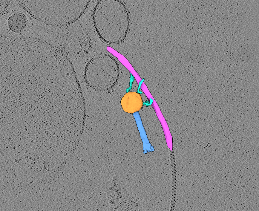
Two raw tilt-series (in MRC format) of highly-purified jumbo bacteriophage in association with bacterial flagella. MDOC files are also provided.
Data DOI: 10.15785/SBGRID/1263 | Publication DOI: doi.org/10.1038/s42003-025-09319-7 | Published: 21 Apr 2026
Briegel Laboratory, Institut Pasteur
Jumbo bacteriophages are exceptionally large viruses that infect bacteria. They consist of a protein shell, or capsid, that encloses the phage DNA genome, along with a tail and baseplate that mediate attachment to the host cell. The Agrobacterium bacteriophage 7-1-1 is a jumbophage capable of binding to bacterial flagella, which it uses to move along the filament toward the cell body prior to infection. This dataset contains tilt-series data of bacteriophage 7-1-1 particles interacting with long bacterial flagellar filaments.
EMPIAR author information: Noteborn WEM, Hoeksma T, Rouchen OY, Briegel A
Paper DOI: https://doi.org/10.1038/s42003-025-09319-7
EMPIAR deposition: EMPIAR-13014
SBGrid CryoET ChallengeBank DOI: 10.15785/SBGRID/1263
Why this dataset is challenging:
Time to completion: ~1.5 days (only 1 day if you choose to use the missing-wedge-corrected tomogram provided rather than compute correction yourself)
Computing required: This guide was made with the intention that an investigator will have access to 4 GPUs. More GPUs is certainly better, and less will mean processing will take longer than the time estimates provided in this guide. The estimates are just rough guides based on our workstation. Ultimately, we leave the computing power dedicated to this tutorial to the discretion of the investigator.
Storage required: 85G (after all the processing is completed).
Software suggested: Multiple software packages need to be used to complete the entire reconstruction. Investigators are welcome to complete as little or as much of the reconstruction pipeline as desired, and tomograms are available if you would prefer to skip certain steps.
For this dataset, we recommend WarpTools dev36 (5.0.0), Imod/3Dmod (4.11.25), IsoNet (0.3), mod2mrc and UCSF ChimeraX (1.1_rhel9).
This dataset contains 2 tilt-series of highly-purified jumbo bacteriophage 7-1-1 and long bacterial flagella filaments. This tutorial guides the user through the reconstruction process of producing tomograms, performing missing wedge correction and manually segmenting a phage and flagella filament.
We will be following the basic steps of tomographic reconstruction:
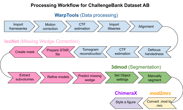
If you have not already downloaded the data, open a command terminal window and type the following command:
rsync -av rsync://challengebank.sbgrid.org/10.15785/SBGRID/1263Check the integrity of the download by assessing if all the components are correctly downloaded to your computer. This pack should contain .tif images, .mdocs, a gain.mrc, and a copy of these instructions.
Download the processing bundle
New tomographers are often confused about the difference between a frame series, a movie, a micrograph and a tilt series. If you know these terms, skip to the next section. If you’re unsure, keep reading.
When a dataset is collected on the microscope, a short movie is taken by exposing the sample to a certain dose of electrons over a certain period of time. The dose is fractionated into frames over the time taken to collect the movie. The movie is therefore composed of a series of frames, called a frame series. The sample stage is then tilted in the microscope in preparation for collecting the next movie (or frame series). At the end of data collection, you will have a collection of movies, each taken at a different discrete angle. The whole collection of movies/frame series acquired across the tilt range constitutes the raw tilt-series data. After motion correction and summing, each frame series yields one tilt image (micrograph) because (almost) all the subframes get summed together to increase the contrast in the image.
Create a workspace. Before we begin, we need to set up a clean workspace for us to be able to work from.
mkdir dataset_AB to make a new directory called “dataset_AB”cd dataset_AB to move into the new directoryln -s /path/to/tutorial/data ./ to create a link to your dataWarpTools create_settings \
--output warp_frameseries.settings \
--folder_processing warp_frameseries \
--folder_data data/ \
--extension "*.mrc" \
--angpix 3.28 \
--bin 0 \
--exposure 2.05Special note: The provided mdoc file refers to the post-aligned stack of tiltseries images and is the original document deposited to EMPIAR by the dataset authors. However, the EMPIAR deposition states that the aligned stacks were binned by 2, which means the pixel size is actually half the value reported in the mdoc files.
This script will create a file called warp_frameseries.settings that will be stored in your project directory. This file is a type of XML metadata file that supplies WarpTools with the settings you provided.
In your script:
warp_frameseries.settings./path/to/your/data/. If you can, you can symbolically link the data folder to your working directory.Time to run (run directly in the commandline): Nearly instant.
WarpTools fs_motion \
--settings warp_frameseries.settings \
--grid 1x1x12 \
--averages

WarpTools fs_ctf \
--settings warp_frameseries.settings \
--voltage 300 \
--cs 2.7 \
--amplitude 0.1 \
--defocus_min 3.0 \
--defocus_max 8.0 \
--range_min 30.0 \
--range_max 7.0 \
--use_sum \
--grid 2x2x1
This script will run the motion correction and CTF estimation job in WarpTools and output summed motion corrected averages in a folder called /averages/ inside the /warp_frameseries/ directory. These summed averages are required for the subsequent steps.
In your script:
header command.Time to run (on 4 GPUs): ~5 minutes
WarpTools filter_quality \
--settings warp_frameseries.settings \
--histograms
This script will print histograms to the terminal screen that will allow you to determine if the motion correction and CTF estimation completed as expected. It can be difficult to tell if the histograms are depicting something sensible, so a good rule of thumb is to look for a normal bell-shape distribution across the defocus. We know that we should expect a normal distribution because the sample was progressively tilted in the microscope. In our experience, if something has gone wrong at this stage, WarpTools tends to dump all frames into the last value of the histograms. Unlike in single-particle analysis, you are not able to assess Thon rings using the Linux version of WarpTools.
In your script:
Time to run (run in the terminal): Nearly instant.
WarpTools ts_import \
--mdocs data/ \
--pattern "*mdoc" \
--frameseries warp_frameseries \
--tilt_exposure 2.05 \
--dont_invert \
--override_axis 85 \
--output tomostar
The frame series has now been motion corrected and summed into single frame micrographs, becoming a motion-corrected tilt series. WarpTools needs to import the single frame tilts using an mdoc file so that WarpTools can know what angle each summed tilt was imaged at. Mdoc files record the angle of each frame series, and since the tilt series have the same file name, WarpTools is able to determine the associated tilt angle.
In your script:
.tomostar files. This folder doesn’t exist yet, but WarpTools will make it for you after this job has been completed. (Here: tomostar.)Time to run (run in the terminal): Nearly instant.
WarpTools create_settings \
--output warp_tiltseries.settings \
--folder_processing warp_tiltseries \
--folder_data tomostar \
--extension "*.tomostar" \
--angpix 3.28 \
--bin 0 \
--exposure 2.05 \
--tomo_dimensions 5600x4200x2200
This script will create a settings file that defines the relevant parameters related to the tilt series. The settings are all the same. If you wanted to bin your pixel size, but you didn’t bin it from the start, now would be your chance to bin the pixel size to speed up processing. Tomostar files will be made for every tiltseries in the dataset and stored in the /tomostar/ folder in the working directory. When it comes time to reconstruct tomograms, WarpTools will fetch information about the tiltseries for reconstruction from the tomostar files.
In your script:
warp_tiltseries.settings.Time to run (run in the terminal): Less than a minute.
WarpTools ts_aretomo3 \
--settings warp_tiltseries.settings \
--angpix 10 \
--patches 6,4 \
--axis 85
WarpTools has a wrapper for the alignment tool AreTomo3. This script will call AreTomo3 to compute the alignment shifts needed to create a smooth, jitter-free aligned series of tilts. Alignment files will be stored in /warp_tiltseries/tiltstack/ under a series of subdirectories with the tomoname label of each tiltseries in the dataset.
In your script:
Time to run (on 4 GPUs): ~5 minutes.
WarpTools ts_defocus_hand \
--settings warp_tiltseries.settings \
--check
This script will compute whether the defocus handedness of the data correlates with the expected CTF model. The result of this quick test will tell us if we need to change any settings related to the defocus handedness.
Time to run (run in the terminal): Nearly instant.
WarpTools ts_defocus_hand \
--settings warp_tiltseries.settings \
--set_noflip
This script will change our settings so that the defocus handedness (the sign value associated with the defocus) is not flipped.
Time to run (run in the terminal): Nearly instant.
WarpTools ts_ctf \
--settings warp_tiltseries.settings \
--defocus_min 3.0 --defocus_max 8.0 \
--range_low 30.0 --range_high 7.0 \
--voltage 300 --cs 2.7 --amplitude 0.1
This script performs 3D CTF correction using the 2D CTF estimation job for the frame series as an initial estimate. Here, we provide all the same values as last time.
In your script:
All parameters are the same as in our previous CTF estimation job.
Time to run (run in the terminal): ~5 minutes
WarpTools ts_reconstruct \
--settings warp_tiltseries.settings \
--angpix 10.0 \
--dont_invert \
--deconv \
--deconv_strength 0.7 \
--deconv_falloff 0.7 \
--perdevice 2
This script will reconstruct the tomogram by direct Fourier-inversion using the alignment information from the AreTomo3 job and the settings stored in the tilt series settings file (tomogram dimensions, etc), and the tiltseries information in the tomostar files. It will output filtered and unfiltered tomograms in /warp_tiltseries/reconstruction/ and /warp_tiltseries/reconstruction/deconv/, respectively.
In your script:
Time to run (run in the terminal): ~10 minutes
This step performs missing wedge correction using IsoNet. The effect of this procedure is to reverse some of the smearing effect in the tomograms along the Z-axis caused by the missing wedge of spatial frequencies in the Fourier transform of the tomogram. The missing wedge is caused by not completely imaging our specimens from all viewing directions, but rather, imaging only at a subset of discrete angles. In practice, without correcting the missing wedge, objects which are spherical (or in our case, icosahedral) become distorted relative to the Z-axis (see screenshot below). After missing wedge correction, our viral capsids will become more icosahedral as one would expect. However, it is important to maintain realistic expectations about what these missing wedge correction programs are able to achieve. In practice, these tools improve the corruption of the image caused by the missing wedge, but they do not remove the corruption completely.
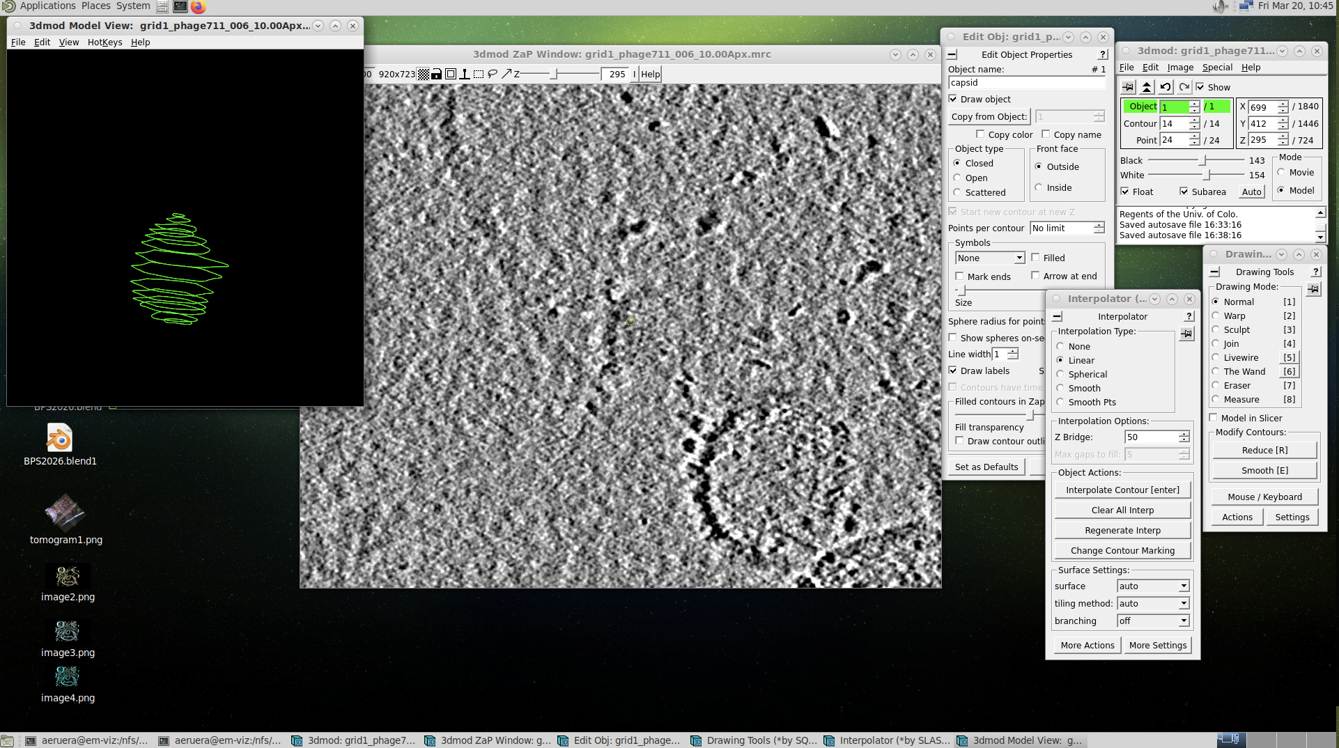
(This is optional, but it’s a good idea to keep results from different programs separated.)
Make a new directory:
mkdir isonetMove into the directory:
cd isonetcp ../warp_tiltseries/reconstruction/deconv/grid1_phage711_006_10.00Apx.mrc .This will copy the deconvolved tomogram (006) from the deconv folder into the current directory.
mv grid1_phage711_006_10.00Apx.mrc grid1_phage711_006_10_00Apx.mrcThe refine step in IsoNet is unable to parse tomogram names which have two dots in them (i.e. _10.00Apx.mrc). In fact, there are several cryoET tools which are not compatible with the standard naming conventions of tomograms produced in WarpTools. Luckily, the pixel size suffix is easy enough to rename. If you have a very large dataset, you may want to script a little Python script to manage renaming large numbers of tomograms.
lsSegmentation is the process of delineating a structure within a tomogram to produce a binary volume. There are many automated segmentation tools available, like MemBRAIN-seg, TARDIS and Easymode. However, they can only segment things the neural networks were trained on. In many cases, when segmenting something niche, the only solution is to manually segment a structure because you may be researching a structure which a) does not belong to the limited number of things that segmentation tools were trained on, or b) is not being adequately segmented by those tools. In this case, phages are not included in these segmentation tool datasets. Further, the capsid fibers that bind to the flagella are long, thin and highly flexible.
In this module, we will take you through how to manually segment a structure in 3DMOD. Once you know how to do it, you will realize it is relatively straight forward and you should be able to segment literally anything in your own tomograms using 3DMOD (i.e. IMOD). As long as you (the human) can see the structure, you can segment it. For this tutorial, we will use 3DMOD to segment the phage capsids, tails, fibers and flagella. This tool is free, reliable and relatively simple. To view this module in action, we have made a YouTube video tutorial to pair with this written guide. (link)
Special note: Manual segmentation involves a lot of clicking and dragging over a prolonged period of time. We recommend regular rest breaks for your wrist, and if possible, an ergonomic mouse.
Concept: Create manual contour lines around objects in the tomogram to segment them. Contours can then be meshed to apply a skin over the top and viewed in ChimeraX as one would with an automated segmentation.
mkdir segmentationcd segmentation3dmod ../isonet/corrected_tomos/l40t05_5_10_00Apx_corrected.mrcThe tomogram will open with an info box and a ZAP window. To get started, we need to check that your mouse settings are correct.
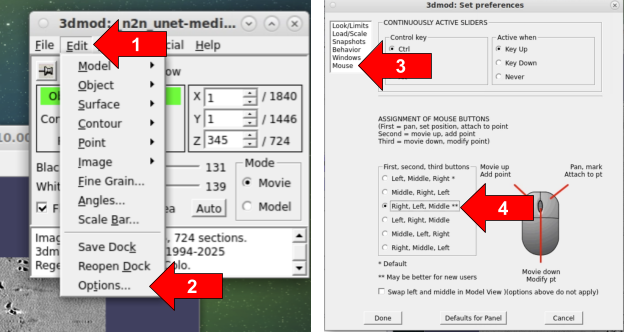
Making sure that the mouse settings are on Right, Left, Middle is strictly so that your mouse settings match those in this instruction guide.
Next, we will edit the settings for our first “Object,” which represents the structure we will segment first. Each structure—the phage capsid, fibers, tail, and flagella—will be segmented as a separate “Object,” so a new object will be created for each structure later. For now, we will focus on Object 1, which is opened by default in 3DMOD.
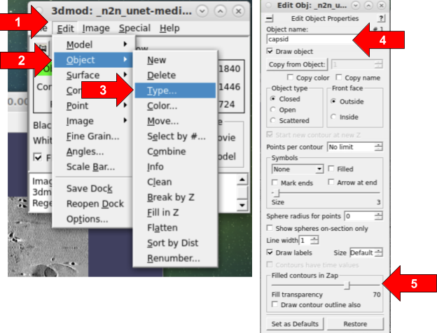
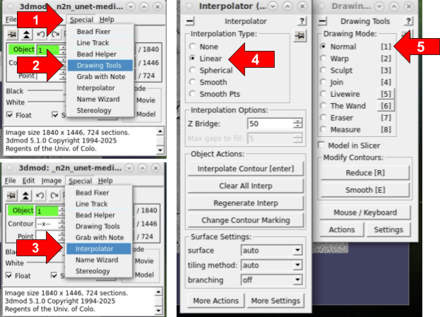
Next, we will open up the drawing tools we need to get started with drawing contours on slices of our tomogram. Once we have the tools set up, we will be ready to start segmenting.
To begin segmenting, you may wish to first zoom in and center a virus in the center of the ZAP window. If you are having trouble distinguishing the boundaries between a structure and the background, it can be helpful to zoom in and zoom out and back in again to allow the human eye to determine edges.
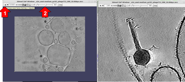
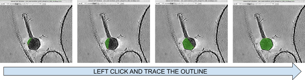
To begin drawing, it’s always easiest to start segmenting from the center of the structure because it’s clearest. Since we are segmenting a capsid, we should slab through the tomogram along the Z (by using the Z slider at the top of the ZAP window) until we roughly locate the center of the capsid. We will then use our left mouse button, and while holding the button down, we will draw a line around the capsid edge.
Tracing carefully around the outside of the capsid, make sure not to fully close the contour by bringing the mouse slightly short of the starting position. If you close the contour, sometimes 3DMOD thinks you were trying to segment everything outside the lines instead of inside the lines. If you make a mistake, you can erase the contour with the ERASE tool in the Interpolator window.
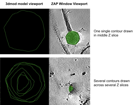
To segment another structure (i.e. the tail, or the flagella), you can create a new Object. You can create as many Objects as you’d like to segment. In theory, you can make them all at the start, and segment all the structures together on each slice as you move through the tomogram, but for the purposes of teaching you the simplest methods, we will create Objects one at a time here. To create a new Object:
Once you have enough contours drawn, you can place a mesh skin over the contour to view the model easier.
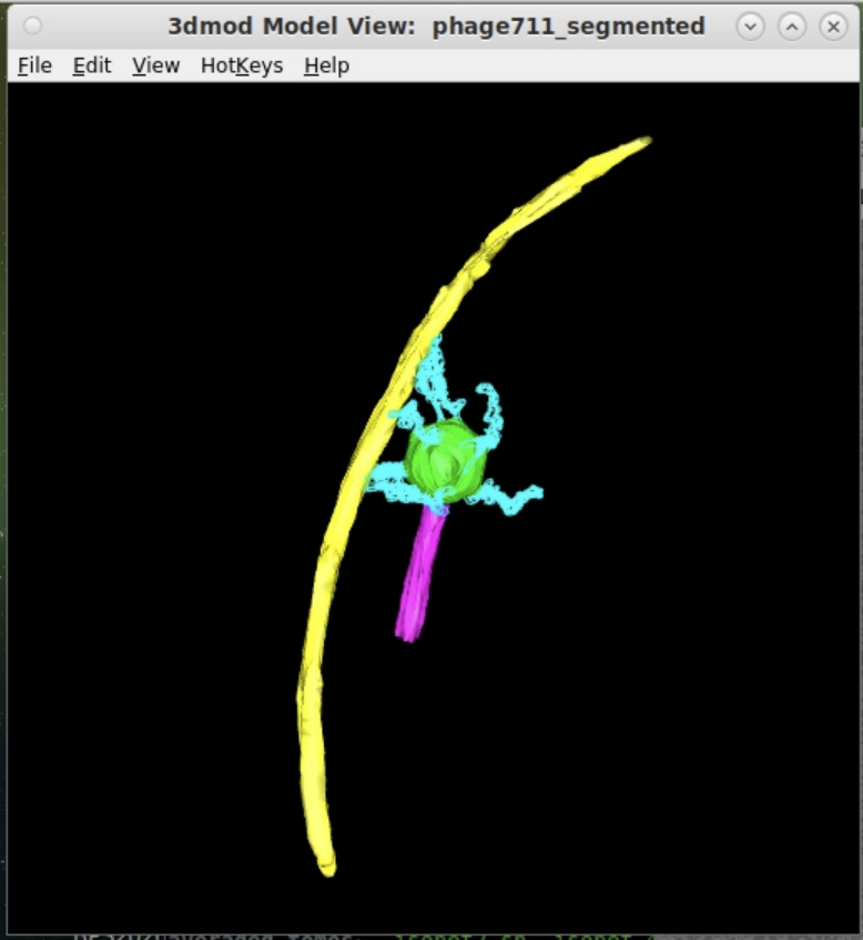
Next, we need to save the model file. We will save it as a .mod file, which IMODs default model file format. To view the .mod file in ChimeraX, we will need to convert it from .mod to .mrc.
To convert from .mod to .mrc, we will use a publicly available mod2mrc script on GitHub: https://github.com/seanhatton/mod2mrc
git clone https://github.com/seanhatton/mod2mrc.git. This will download the script you need into a newly created folder called /mod2mrc/.ls to ensure that the /mod2mrc/ folder is there.mod2mrc folder; cp manually_segmented_phage711.mod /mod2mrc/ followed by cp phage711.mrc /mod2mrc/.cd /mod2mrc/ followed by ls. You should see mod2mrc.bash, readme.txt and the files you copied.input_mrc="phage711.mrc"
input_mod="manually_segmented_phage711.mod"
object_list=(phage711_capsid tail capsid_fibers flagella)*Make sure there are no spaces in the object list name.
chmod +x mod2mrc.bash../mod2mrc.bash.To view segmentations and assess their quality, we can open them in UCSF ChimeraX. Since we have converted to an .mrc format, you can make figures using whatever your preferred rendering software tool is in the usual manner (including Blender and other 3D render applications). To open a segmentation:
chimerax phage711_capsid.mrcWhen UCSF ChimeraX opens, it may load the segmentation as a plane. You will need to adjust the segmentation to be rendered in the Surface representation by clicking the render setting drop down box. You will also need to set the contour level to a value below 1. You can set the render steps to 1. View the YouTube video for more information.
Congratulations on processing the dataset to completion!
This is one way of many potential ways that a dataset of this nature could be processed. New cryoET tools are emerging all the time. You can visit sbgrid.org to view our most updated collection of software titles.
If you have any questions, please contact eruera@hkl.hms.harvard.edu with DATASET AB as the subject line.