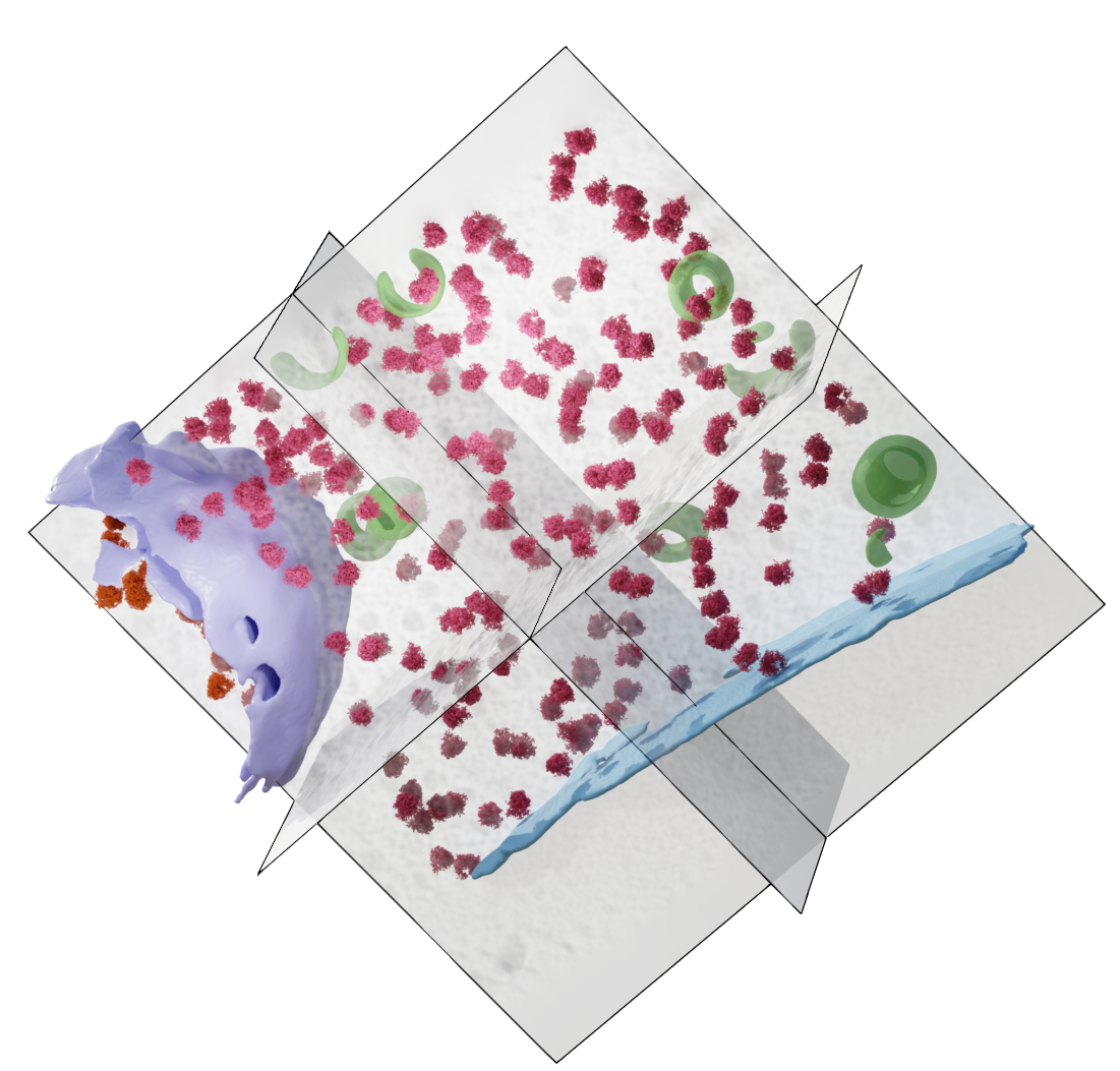
Tilt-series of milled Saccharomyces cerevisiae cells depicting mitochondria, nuclear envelopes, lipid bodies, smooth endoplasmic reticulum and other intracellular components.
Data DOI: 10.15785/SBGRID/1255 | Published: 21 Apr 2026
Raunser Laboratory, Max Planck Institute of Molecular Physiology
For this exercise, we will be processing a small subset of a milled yeast dataset. The data was acquired by the Stefan Raunser group from the Max Planck Institute in Dortmund, Germany. A special thanks to Tatjana Taubitz, Elisa Lisicki, Sebastian Tacke and Stefan Raunser for making the data available. The dataset was collected on a Titan Krios dataset and the original subset contains almost 100 tilt-series of FIB-milled yeast cells.
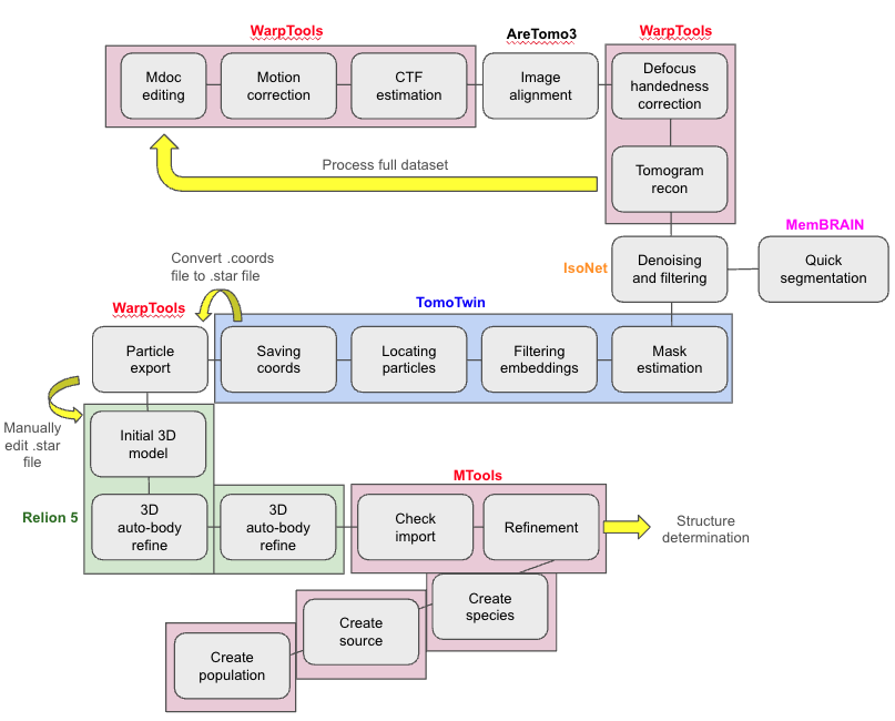
This guide will cover steps from processing raw images such as those obtained directly from the microscope to density maps obtained by subtomogram averaging.
Due to time constraints, we will not be running the full workflow in this workshop. We have prepared pre-calculated results for several steps to speed up the process and reduce computational burden. All principles are applicable to the entirety of the data. Instructions for the full workflow are included, with instructions to indicate changes for running the time-constrained version we will be using.
This exercise is intended for use with Relion 4 (5.0.0_cu12.2) with Napari (0.4.18), Warp (2.0.0dev36), AreTomo3 (2.2.2), IsoNET (0.3), TomoTWIN (0.9.1), and Imod (5.1.3). We will also use the visualization software UCSF ChimeraX version 1.10_rhel9.
(For Relion jobs run in Amazon Web Services (AWS), the slurm errors about _handle_getpw and _handle_getgr can be ignored.)
SBGrid CryoET ChallengeBank DOI: 10.15785/SBGRID/1255
If you have not already downloaded the data, open a command terminal window and type:
rsync -av rsync://challengebank.sbgrid.org/10.15785/SBGRID/1255When not specified, parameter values can be left at their defaults.
In the terminal window, navigate to the working directory for your project:
cd /shared/data/projects/$USER/ or cd /shared/data/projects/tttuserNNNN (replacing the NNNN with your user number)ls. You should see several directories, e.g. 1_warp_scripts, 2_isonet_scripts, etc.cd 1_warp_scriptsFirst, we need to create the settings file that defines our input data and where it is stored.
#!/bin/bash

WarpTools create_settings \
--output warp_frameseries.settings \
--folder_processing ${PWD}/warp_frameseries \
--folder_data /shared/data/projects/${USER}/raw_data/subset3/ \
--extension "*.eer" \
--gain_path /shared/data/projects/${USER}/raw_data/subset3/reference.gain \
--eer_ngroups 42 \
--angpix 1.56 \
--bin 0 \
--exposure 2.41 \
--tomo_dimensions 4400x4400x2200 > warp_create_fs_settings.out 2> warp_create_fs_settings.err
In your script:
/warp_frameseries on the end of the path. (The script will create a subdirectory titled “warp_frameseries”. You do not need to make it yourself.)To run:
./01_warp_create_fs_settings.shTime for one tomogram (CPU only job): A few seconds. After successful completion, the log should show "123 files found"
We need to estimate the motion of our specimen in 2D prior to CTF estimation and correction. Corrected averages will be written out to the /warp_frameseries/average directory as .xml files. There will be one .xml file for every fraction in the tilt-series.
#!/bin/bash
#SBATCH --job-name=warp_motion_ctf
#SBATCH --error=warp_motion_ctf.err
#SBATCH --output=warp_motion_ctf.out
#SBATCH --ntasks=5
#SBATCH --nodes=1
#SBATCH --cpus-per-task=6
#SBATCH --gres=gpu:4
#SBATCH --partition=relion-gpu-medium-mixed

echo "SLURM: ${SLURM_JOB_ID}"

WarpTools fs_motion \
--settings warp_frameseries.settings \
--grid 1x1x5 \
--averages

WarpTools fs_ctf \
--settings warp_frameseries.settings \
--voltage 300 \
--cs 2.7 \
--amplitude 0.1 \
--defocus_min 3.0 \
--defocus_max 8.0 \
--range_min 30.0 \
--range_max 7.0 \
--use_sum \
--grid 2x2x1
To run:
sbatch 02_warp_motion_and_ctf.shTime for one tomogram (4 GPUs): ~10 minutes. After successful completion, the log should show 123/123, 00:00 remaining.
This step is technically optional but we advise not to skip it. It will print histogram plots to the terminal window that you can use to evaluate if the jobs have run correctly. It will inform you how many frames were estimated to contain what degree of CTF fit (e.g. 13 frames at CTF fit of 4.2 - 4.6 A).
#!/bin/bash

WarpTools filter_quality \
--settings warp_frameseries.settings \
--histograms > warp_histograms.out 2> warp_histograms.err
To run:
./03_warp_histograms.shTime for one tomogram (4 GPUs): Nearly instant.
Read the contents of the .out file to view the histograms printed to the terminal.
Tell Warp which files belong to which tiltseries by importing them so that you can manage your data downstream.
#!/bin/bash

WarpTools ts_import \
--mdocs /shared/data/projects/${USER}/raw_data/subset3/ \
--pattern "*.mdoc" \
--frameseries warp_frameseries \
--tilt_exposure 2.41 \
--dont_invert \
--override_axis 84 \
--output tomostar \
--min_intensity 0.8 > warp_ts_import.out 2> warp_ts_import.err
In your script:
To run:
./04_warp_tiltseries_import.shTime for one tomogram (4 GPUs): Instant. After successful completion, the log should show "Successfully parsed 3 MDOC files, 0 failed".
Create a .settings file that tells Warp how to process the tilt series. Produce metadata files (STAR files) based on the original mdoc files (output by SerialEM) that Warp can use to import and manage your data downstream. This is where it becomes important to change the tomogram dimensions if you wished to reconstruct tomograms with a smaller or larger Z-height later (for example, if your dimensions truncated your region of interest).
#!/bin/bash

WarpTools create_settings \
--output warp_tiltseries.settings \
--folder_processing warp_tiltseries \
--folder_data tomostar \
--extension "*.tomostar" \
--angpix 1.56 \
--bin 0 \
--exposure 2.41 \
--tomo_dimensions 4400x4400x2200 > warp_ts_settings.out 2> warp_ts_settings.err
In your script:
To run:
./05_warp_create_ts_settings.shTime for one tomogram (4 GPUs): Instant. After successful completion, the log should show "3 files found".
Align tilt-series images using AreTomo3. The AreTomo3 wrapper in Warp automates running AreTomo3 by preparing inputs, passing parameters, and reintegrating outputs into Warp’s workflow.
#!/bin/bash
#SBATCH --job-name=warp_aretomo3
#SBATCH --error=warp_aretomo3.err
#SBATCH --output=warp_aretomo3.out
#SBATCH --ntasks=5
#SBATCH --nodes=1
#SBATCH --cpus-per-task=6
#SBATCH --gres=gpu:4
#SBATCH --partition=relion-gpu-medium-mixed

echo "SLURM: ${SLURM_JOB_ID}"

WarpTools ts_aretomo3 \
--settings warp_tiltseries.settings \
--angpix 10 \
--patches 6,4 \
--output_processing aretomo3 \
--axis 84
In your script:
header $name.mdoc into the terminal. For other projects, if you don’t know the tilt angle axis, you can omit the --axis 84 parameter and input --axis_batch 3 and --axis_iter to ask AreTomo3 to refine the tilt axis angle. AreTomo3 will try to guess by running an automatic tilt-angle search.)To run:
sbatch 06_aretomo3_alignment.shTime for one tomogram (3 GPUs): ~5 minutes.
You cannot check the aligned mrc files for AreTomo3 because it does not output any. You can check how well it performed at the tomogram stage. After successful completion, the log should show "3/3, 00:00 remaining".
Inside the microscope, “defocus” is the distance between the sample plane and the focal plane of the objective lens. The image can be focused above or below the specimen (positive or negative sign convention). If the wrong handedness is used, CTF oscillations will get flipped and phases will be inverted incorrectly. Warp helps you check the defocus handedness using this script.
#!/bin/bash

WarpTools ts_defocus_hand \
--settings warp_tiltseries.settings \
--check > warp_check_defocus.out 2> warp_check_defocus.err
To run:
./07_warp_check_defocus.shTo inspect the result, run:
You will see the following; “The average correlation is negative, which means that the defocus handedness should be set to 'flip'.”
Time for one tomogram (4 GPUs): < 30 seconds.
We need to set the defocus handedness by saving the ‘flip’ setting into the settings file.
#!/bin/bash

WarpTools ts_defocus_hand \
--settings warp_tiltseries.settings \
--set_flip > warp_set_defocus.out 2> warp_set_defocus.err
To run:
./08_warp_set_defocus.shTime for one tomogram (4 GPUs): < 5 seconds. After successful completion, the log should show "Setting defocus handedness to 'flip' for all tilt series… 3/3".
Warp performs CTF correction by estimating the defocus and astigmatism for each tilt image (performed earlier) and mathematically compensating for the phase distortions introduced by the microscope’s optics. This improves image contrast and restores high-frequency details and makes downstream reconstruction and averaging more accurate.
#!/bin/bash

WarpTools ts_ctf \
--settings warp_tiltseries.settings \
--defocus_min 3.0 \
--defocus_max 8.0 \
--range_low 30.0 \
--range_high 7.0 \
--voltage 300 \
--cs 2.7 \
--amplitude 0.1 > warp_ctf_correction.out 2> warp_ctf_correction.err
To run:
./09_warp_ctf_correction.shTime for one tomogram (4 GPUs): ~1 minute. After successful completion, the log should show "3/3, 00:00 remaining".
Reconstruct tomograms in .mrc format using the parameters set in the settings file. The time this will take depends on the size of the tomogram dimensions and the --angpix variable.
Reconstruct tomograms from the AreTomo3 alignment.
#!/bin/bash
#SBATCH --job-name=warp_reconstruction
#SBATCH --error=warp_reconstruction.err
#SBATCH --output=warp_reconstruction.out
#SBATCH --ntasks=5
#SBATCH --nodes=1
#SBATCH --cpus-per-task=6
#SBATCH --gres=gpu:4
#SBATCH --partition=relion-gpu-medium-mixed

WarpTools ts_reconstruct \
--settings warp_tiltseries.settings \
--input_processing aretomo3/ \
--angpix 10.0 \
--dont_invert \
--deconv \
--deconv_strength 0.7 \
--deconv_falloff 0.7 \
--perdevice 1
In your script:
To run:
sbatch 10_warp_reconstruction.shTime for one tomogram (4 GPUs): ~5 minutes. After successful completion, the log should show "3/3, 00:00 remaining".
To inspect the quality of a tomogram, navigate to the output folder where the tomograms are stored;
cd aretomo3/reconstruction/imod $tomoname.mrc.imod $your_tomo.mrcAdjust the master script so that we can reconstruct the remaining tilt-series in the datasets provided using a one-stop-shop Warp script. We need to:
aretomo3/reconstruction/ directory with cd ../../sbatch warp_workflow.sh#!/bin/bash
#SBATCH --job-name=warp_workflow
#SBATCH --error=warp_workflow.err
#SBATCH --output=warp_workflow.out
#SBATCH --ntasks=5
#SBATCH --nodes=1
#SBATCH --cpus-per-task=6
#SBATCH --gres=gpu:4
#SBATCH --partition=relion-gpu-medium-mixed
WarpTools create_settings \
--output warp_frameseries.settings \
--folder_processing /shared/data/projects/${USER}/1_warp_scripts/warp_frameseries \
--folder_data /shared/data/projects/${USER}/raw_data/subset7/ \
--extension "*.eer" \
--gain_path /shared/data/projects/${USER}/raw_data/subset7/reference.gain \
--eer_ngroups 42 \
--angpix 1.56 \
--bin 0 \
--exposure 2.41 \
--tomo_dimensions 4400x4400x2200
WarpTools fs_motion \
--settings warp_frameseries.settings \
--grid 1x1x5 \
--averages
WarpTools fs_ctf \
--settings warp_frameseries.settings \
--voltage 300 \
--cs 2.7 \
--amplitude 0.1 \
--defocus_min 3.0 \
--defocus_max 8.0 \
--range_min 30.0 \
--range_max 7.0 \
--use_sum \
--grid 2x2x1
WarpTools filter_quality \
--settings warp_frameseries.settings \
--histograms
WarpTools ts_import \
--mdocs /shared/data/projects/${USER}/raw_data/subset7/ \
--pattern "*.mdoc" \
--frameseries warp_frameseries \
--tilt_exposure 2.41 \
--dont_invert \
--override_axis 84 \
--output tomostar \
--min_intensity 0.8
WarpTools create_settings \
--output warp_tiltseries.settings \
--folder_processing warp_tiltseries \
--folder_data tomostar \
--extension "*.tomostar" \
--angpix 1.56 \
--bin 0 \
--exposure 2.41 \
--tomo_dimensions 4400x4400x2200
WarpTools ts_aretomo3 \
--settings warp_tiltseries.settings \
--angpix 10 \
--patches 6,4 \
--output_processing aretomo3 \
--axis 84
WarpTools ts_defocus_hand \
--settings warp_tiltseries.settings \
--set_flip
WarpTools ts_ctf \
--settings warp_tiltseries.settings \
--defocus_min 3.0 \
--defocus_max 8.0 \
--range_low 30.0 \
--range_high 7.0 \
--voltage 300 \
--cs 2.7 \
--amplitude 0.1
WarpTools ts_reconstruct \
--settings warp_tiltseries.settings \
--input_processing aretomo3/ \
--angpix 10.0 \
--dont_invert \
--deconv \
--deconv_strength 0.7 \
--deconv_falloff 0.7 \
--perdevice 1View the reconstructed tomograms by navigating to ./aretomo3/reconstruction/ and opening the tomograms in IMOD;
imod *.mrcMrcConverter --reverse in the terminal to convert the tomograms if needed.To denoise tomograms and improve the visual appearance of low-signal features, we can perform CTF deconvolution and missing wedge correction in IsoNet. IsoNet has a graphical user interface (which you can launch by typing isonet.py gui in the command line, but for the purposes of this tutorial, we will run IsoNet in the command line.)
We will run IsoNet on only one tomogram to save time in this workshop using a pre-calculated IsoNet model that we prepared for you. We provide you with all the pre-denoised tomograms later. If you want to know how to create a model yourself from your own data, you can follow our instruction guide here.
We have prepared an IsoNet model for you. You will need to first navigate to the new isonet working directory (/shared/data/projects/${USER}/2_isonet_scripts/).
cp /shared/data/projects/${USER}/1_warp_scripts/aretomo3/reconstruction/$tomoname.mrc . Your isonet folder should now have the following items in it:
l40t05_5_10.00Apx.mrc)pre_trained_modelsPrepare a tomograms.star file.
#!/bin/bash

isonet.py prepare_star ${PWD} --output_star tomograms.star --pixel_size 10.0 > isonet_prep.out 2> isonet_prep.err
Note: provide only the path to the directory. Don’t include the name of the .mrc file.
To run:
./1_isonet_prepare_starfile.shTime for one tomogram (CPU only): near instant
In real life, this step is optional but for this tutorial, we demonstrate deconvolution in IsoNet.
#!/bin/bash

isonet.py deconv tomograms.star --snrfalloff 0.7 --deconv_folder deconv > isonet_deconv.out 2> isonet_deconv.err
To run:
./2_isonet_deconvolute.shTime for one tomogram (1 GPUs): 1-2 minutes
deconv directory and open the tomogram in IMOD to inspect how well IsoNet performed the filtering. (For those interested, you could compare the performance of Warps in-built deconvolution and IsoNets deconvolution.)#!/bin/bash
#SBATCH --job-name=isonet_predict
#SBATCH --ntasks=1
#SBATCH --nodes=1
#SBATCH --cpus-per-task=12
#SBATCH --gres=gpu:4
#SBATCH --partition=relion-gpu-medium-mixed
#SBATCH --error=isonet_predict.err
#SBATCH --output=isonet_predict.out
MDL=/shared/data/projects/et-models/isonet/model_iter15.h5
echo "SLURM: ${SLURM_JOB_ID}"
# help text mentions that gpuID is optional, but fails with an error to detect GPUs if not specified
isonet.py predict tomograms.star ${MDL} --gpuID 0,1,2,3To run:
sbatch 3_isonet_predict.shTime for one tomogram (GPU only): 15 minutes
We will cover (very briefly) the simple MemBRAIN-seg program for tomogram segmentation. For this workflow, we will use the denoised tomograms we already produced. MemBRAIN-seg works best on denoised tomograms.
cd /shared/data/projects/${USER}/3_membrain_scriptscp /shared/data/projects/${USER}/2_isonet_scripts/corrected_tomos/*_corrected.mrc .Example slurm submission script for 1_membrain_segment.sh:
#!/bin/bash
#SBATCH -n 1
#SBATCH -N 1
#SBATCH -c 12
#SBATCH --gres=gpu:4
#SBATCH --partition=relion-gpu-medium-mixed
#SBATCH --error=membrain_seg.err
#SBATCH --output=membrain_seg.out
#SBATCH --job-name=membrain_seg

#Tomogram path must be a complete path and needs to include the name of the file.
#ckpt-path must be an absolute path to the ckpt model.

TOMO_NAME=l40t05_5_10.00Apx_corrected.mrc
#Make sure to alter the tomoname above to match your tomogram

MDL=/shared/data/projects/et-models/membrain/MemBrain_seg_v10_beta.ckpt

echo "SLURM: ${SLURM_JOB_ID}"

membrain segment --tomogram-path ${PWD}/${TOMO_NAME} \
--ckpt-path ${MDL} \
--out-folder .
IMPORTANT: --tomogram-path needs a full path and must include the name of the tomogram. It cannot parse relative paths.
In your script:
To run:
sbatch 1_membrain_segment.shTime for one tomogram (GPU only): 10 minutes
Check the segmentation by opening the .mrc output in either UCSF ChimeraX or IMOD.
We can compare the difference between segmentation results from an undenoised tomogram and a tomogram denoised in IsoNet. We have prepared this for you. View the two tomograms in:
/shared/data/projects/cryoet-data/data_for_participants20251022/precalculated_memBRAIN_results/undenoised_vs_denoised_segmentations/
In this tutorial, we will only be picking particles on a single down-sampled tomogram. We will provide you with pre-calculated results for the rest of the dataset. This is the primary reason why we reconstructed tomograms with a tomo pixel size of 10 angstroms as TomoTWIN is designed to work with tomograms of that size.
To speed up processing, we have provided you with a pre-trained model (cluster_targets.temb) that you will use to pick on your favourite tomogram in the dataset.
cp /shared/data/projects/${USER}/2_isonet_scripts/*.mrc /shared/data/projects/${USER}/4_tomotwin_scripts/pre-trained/cp /shared/data/projects/${USER}/2_isonet_scripts/corrected_tomos/*_corrected.mrc /shared/data/projects/${USER}/4_tomotwin_scripts/pre-trained/cd /shared/data/projects/${USER}/4_tomotwin_scripts/pre-trained/cluster.temb file.Estimate a mask that covers the region of interest and excludes the void (empty space above and below the tomogram). This will allow TomoTwin to focus on the areas of the tomogram that are likely to include your specimen.
Adjust script 1_tomotwin_mask_estimate.sh by opening it in geany.
geany 1_tomotwin_mask_estimate.sh#!/bin/bash
#SBATCH --job-name=tomotwin_mask
#SBATCH --ntasks=1
#SBATCH --nodes=1
#SBATCH --cpus-per-task=12
#SBATCH --gres=gpu:4
#SBATCH --partition=relion-gpu-medium-g5
#SBATCH --error=tomotwin_mask.err
#SBATCH --output=tomotwin_mask.out
MDL=/shared/data/projects/et-models/tomotwin/tomotwin_latest.pth
INMRC=l40t05_5_10.00Apx.mrc
echo "SLURM: ${SLURM_JOB_ID}"
tomotwin_tools.py embedding_mask median \
-i ${INMRC} \
-m ${MDL} \
-o maskIMPORTANT: Supply your undenoised tomogram for this step.
In your script:
/mask/.To run:
sbatch 1_tomotwin_mask_estimate.shTime for one tomogram (4 GPUs): 10 minutes.
Filter the embeddings (2D vectors that represent signals present in small 3D patches of the tomogram) using the mask you estimated to define the region of interest.
Adjust script 2_tomotwin_filtering_embeddings.sh by opening it in geany.
geany 2_tomotwin_filtering_embeddings.sh#!/bin/bash
#SBATCH --job-name=tomotwin_filteringembed
#SBATCH --ntasks=1
#SBATCH --nodes=1
#SBATCH --cpus-per-task=48
#SBATCH --gres=gpu:4
#SBATCH --partition=relion-gpu-medium-g5
#SBATCH --error=tomotwin_filteringembed.err
#SBATCH --output=tomotwin_filteringembed.out
MDL=/shared/data/projects/et-models/tomotwin/tomotwin_latest.pth
INMRC=l40t05_5_10.00Apx.mrc
INMSK=mask/l40t05_5_10.00Apx_mask.mrc
echo "SLURM: ${SLURM_JOB_ID}"
tomotwin_embed.py tomogram -v ${INMRC} \
-m ${MDL} \
--mask ${INMSK} \
-o out/embed/tomo/ \
-s 2IMPORTANT: Supply your undenoised tomogram for this step.
In your script:
To run:
sbatch 2_tomotwin_filter_embeddings.shTime for one tomogram (4 GPUs): 30 minutes.
We provide you with a pre-calculated target embedding file to save time. This embedding file represents the expected embeddings from representative ribosomes picked from this dataset. Step 3 will take the embeddings from subvolumes in your tomogram and compare them to the target embeddings, and generate a localization map.
Adjust script 3_tomotwin_map_tomo.sh by opening it in geany.
geany 3_tomotwin_map_tomo.sh#!/bin/bash
INEMB=out/embed/tomo/l40t05_5_10.00Apx_embeddings.temb
#Make sure to update the tomoname above to match your tomoname.
tomotwin_map.py distance -r cluster_targets.temb \
-v ${INEMB} \
-o out/map/ > tomotwin_map_tomo.out 2> tomotwin_map_tomo.errIn your script:
We have provided you with the cluster_targets.temb file for your convenience. It takes about an hour to produce one of these, but the procedure is relatively simple.
To run:
./3_tomotwin_map_tomo.shTime for one tomogram (CPU only): A few seconds.
Locate potential particles within the tomogram.
Adjust script 4_tomotwin_locate_particles.sh by opening it in geany.
geany 4_tomotwin_locate_particles.sh#!/bin/bash
#SBATCH --job-name=tomotwin_locate_particles
#SBATCH --ntasks=1
#SBATCH --nodes=1
#SBATCH --cpus-per-task=12
#SBATCH --gres=gpu:4
#SBATCH --partition=relion-gpu-medium-g5
#SBATCH --error=tomotwin_locate_particles.err
#SBATCH --output=tomotwin_locate_particles.out
echo "SLURM: ${SLURM_JOB_ID}"
tomotwin_locate.py findmax -m out/map/map.tmap -o out/locate/In your script:
/out/map/map.tmap.To run:
sbatch 4_tomotwin_locate_particles.shTime for one tomogram (4 GPUs): 5 minutes.
Visualize and set an appropriate threshold that includes particle picks of your interest and minimal membrane picks.
IMPORTANT: Supply your denoised tomogram for this step. It will help you visualize the contents of the tomogram.
Open the tomogram and the locate.tloc file in napari_boxmanager.
napari_boxmanager $tomoname_corrected.mrc out/locate/located.tloccoords.tloc.The coordinates are saved in a tloc file. This file needs to be converted into a coordinate file and then converted from there into a STAR file for WarpTools export.
Adjust script 5_tomotwin_convert_tloc.sh by opening it in geany.
geany 5_tomotwin_convert_tloc.sh#!/bin/sh
tomotwin_pick.py -l coords.tloc -o coords/ > tomotwin_convert_tloc.out 2> tomotwin_convert_tloc.errIn your script:
Time for one tomogram (CPU only): instant.
Check the presence of the .coords files in the coords/ folder. Rename the .coords file with tomoname. For example, from cluster_1.coords, type mv cluster_1.coords l40t05_5.coords to rename the file to l40t05_5.coords. Rename it after your tomogram, and leave it in the coords/ subdirectory.
Convert the coords file to a Warp-compatible STAR file with appropriate formatting using a python script. Make sure the coords are named after the tomogram you picked them on, minus the pixel size suffix. For example, if the tomogram is called l40t05_5_10.00Apx.mrc, then the coordinate file needs to be renamed to l40t05_5.coords. The name of the coords file is used to populate the _rlnMicrographName column of the STAR file with the correct tomoname and a .tomostar suffix. This formatting is required for WarpTools.
Rename the coords file after the tomoname. Then, run the script from the main /4_tomotwin_scripts/ directory.
./tomotwin_coords_to_warp.pyTime for one tomogram (in terminal window): instant.
End of Day One. Stop here and transfer to the pre-calculated folder for Day Two.
Warp will take the particle coordinates and use them to reconstruct 3D or 2D subvolumes de novo from the tiltseries settings and corrections information stored in the Warp working directory.
Navigate back to the working directory.
cd /shared/data/projects/${USER}/nov6_subset7/#!/bin/bash
WarpTools ts_export_particles \
--settings warp_tiltseries.settings \
--input_star particle_coordinates.star --normalized_coords \
--output_angpix 4.70 --box 128 --diameter 250 \
--output_processing subtomograms \
--output_star relion/particles_warp.star --2d \
--relative_output_paths > warp_export.out 2> warp_export.errIn your script:
/aretomo3/ inside a subdirectory called /particlesseries/.To run:
./1a_WarpTools_export_particles.shTime for one tomogram (4 GPUs): ~1m.
This will output 2D subvolumes in a subdirectory called subtomograms. You can check them by viewing the summed average mrc files in IMOD.
Subvolumes containing putative particles extracted from the reconstructed tomogram are subjected to iterative alignment procedures to rotate and translate them in 3D space to maximize cross-correlation with a reference. Through successive cycles of alignment and averaging, stochastic noise is reduced while coherent structural features are reinforced. This process is identical to the 3D volume refinement process in single-particle EM.
At this point in the workshop, to keep jobs within a reasonable runtime, we will continue with a smaller particle subset which will unfortunately limit the resulting resolution. Several steps (Bayesian Polishing, CTF Refinement, Re-extracting refined particles) are not meaningful at these resolutions but may be appropriate for other datasets.
Edit the optimisation_set.star file that WarpTools outputs. There is a missing file name in this star file which must be input manually.
cd relion or cd /shared/data/projects/${USER}/nov6_subset7/relion)geany particles_warp_optimisation_set.starparticles_warp.star into the _rlnTomoParticlesFile column of the star file.
From within the relion/ folder, launch the Relion 5 GUI:
relion --tomo &particles_warp_optimisation_set.star.When the job has run for a while, evaluate your 3D refinement by opening the run_it$$$_class001.mrc volume in UCSF ChimeraX. It should look like a terrible ribosome.
We will abort this job early before it finishes to save time, once we have acquired a reference good enough to progress to Refine3D.
From within the Relion 5 GUI;
particles_warp_optimisation_set.star.InitialModel/job001/run_it$$$_class001.mrc.When the job has run for a while, evaluate your 3D refinement by opening the run_it$$$_class001.mrc volume in UCSF ChimeraX. It should look like a ribosome!
Moving forward, we will use pre-calculated RELION results to save time (this Refine3D job would otherwise take over an hour to run to completion).
2D particles that have been aligned in Relion 5 to a decent volume reconstruction can then be fed into MTools for further refinement. MTools will return to the settings used in WarpTools and use the new particle coordinates and alignment information/poses to calculate per-particle defocus and CTF correction before performing its own refinement procedure. In a high-resolution pipeline, refinements would be made in Relion and MTools iteratively with progressive un-binning until resolution ceases to improve. These steps should be performed in the /shared/data/projects/${USER}/nov6_subset7 precalculated project directory, not the relion subdirectory, so that MTools is able to locate the relative WarpTools files it requires.
Create a population in MTools with 1_MTools_create_population.sh.
#!/bin/bash

MTools create_population \
--directory m_run01 \
--name population_01 > MTools_create_population.out 2> MTools_create_population.err
In your script:
To run:
./1_MTools_create_population.shTime for one tomogram (CPU only): A few seconds.
Create a source in MTools with 2_MTools_create_source.sh.
#!/bin/bash

MTools create_source \
--population m_run01/population_01.population \
--processing_settings warp_tiltseries.settings \
--name source_01 > MTools_create_source.out 2> MTools_create_source.err
In your script:
To run:
./2_MTools_create_source.shTime for one tomogram (CPU only): A few seconds.
Create a species in MTools with 3_MTools_create_species.sh.
#!/bin/bash
#SBATCH --job-name=MTools_create_species
#SBATCH --error=MTools_create_species.err
#SBATCH --output=MTools_create_species.out
#SBATCH --ntasks=5
#SBATCH --nodes=1
#SBATCH --cpus-per-task=6
#SBATCH --gres=gpu:1
#SBATCH --partition=relion-gpu-medium-g5

echo "SLURM: ${SLURM_JOBID}"

MTools create_species \
--population m_run01/population_01.population \
--name species_01 \
--diameter 250 \
--sym C1 \
--temporal_samples 1 \
--particles_relion relion/Refine3D/job002/run_data.star \
--half1 relion/Refine3D/job002/run_half1_class001_unfil.mrc \
--half2 relion/Refine3D/job002/run_half2_class001_unfil.mrc \
--mask binary_mask_ribosome_box128_apix4.70.mrc \
--angpix 4.70 \
--angpix_resample 4.70
In your script:
To run:
sbatch 3_MTools_create_species.shTime for one tomogram (CPU only): ~40 minutes.
Refine in MCore without any iterations with 4_MTools_MCore_1.sh.
#!/bin/bash
#SBATCH --job-name=MTools_mcore_1
#SBATCH --error=MTools_mcore_1.err
#SBATCH --output=MTools_mcore_1.out
#SBATCH --ntasks=5
#SBATCH --nodes=1
#SBATCH --cpus-per-task=6
#SBATCH --gres=gpu:4
#SBATCH --partition=relion-gpu-medium-g5

echo "SLURM: ${SLURM_JOBID}"

MCore \
--population m_run01/population_01.population \
--iter 0 \
--perdevice_refine 1 --port -1
In your script:
To run:
sbatch 4_MTools_MCore_1.shTime for one tomogram (CPU only): ~10m
Refine in MCore with iterations with 5_MTools_MCore_2.sh.
#!/bin/bash
#SBATCH --job-name=MTools_mcore_2
#SBATCH --error=MTools_mcore_2.err
#SBATCH --output=MTools_mcore_2.out
#SBATCH --ntasks=5
#SBATCH --nodes=1
#SBATCH --cpus-per-task=6
#SBATCH --gres=gpu:1
#SBATCH --partition=relion-gpu-medium-g5

echo "SLURM: ${SLURM_JOB_ID}"

MCore \
--population m_run01/population_01.population \
--refine_imagewarp 6x4 \
--refine_particles \
--ctf_defocus \
--ctf_defocusexhaustive \
--perdevice_refine 1
In your script:
To run:
sbatch 5_MTools_MCore_2.shTime for one tomogram (CPU only): ~3m